Markowitz minimum-variance portfolio: a quadratic programming example, solved and checked
The Markowitz minimum-variance portfolio is a classic quadratic programming problem. Here it is solved by a real solver (CLARABEL) and checked: every constraint, the dual, and the optimality certificate. Change the numbers below and solve your own.
Solve your own version free, no account needed
Say it or snap it
You can give ProvenDecisions this problem out loud or as a photo. The app wrote down both, solved them, and got the same checked answer as the typed version.
What the app heard: “3 assets have expected returns of 8, 12 and 15 percent and volatilities of 10, 20 and 30 percent. The correlation is 0.2 between assets 1 and 2, 0.1 between assets 1 and 3, and 0.3 between assets 2 and 3. Invest all the money with no short sales and an expected return of at least 11 percent. Minimize the portfolio variance.”
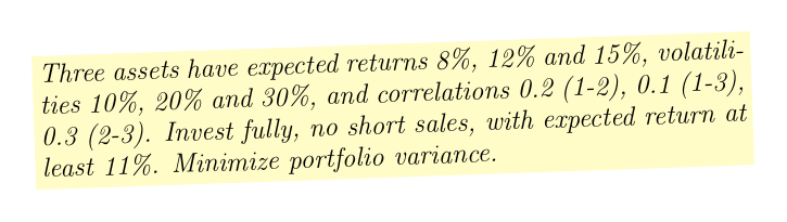
The problem
Three assets have expected returns 8%, 12% and 15%, volatilities 10%, 20% and 30%, and correlations 0.2 (1-2), 0.1 (1-3), 0.3 (2-3). Invest fully, no short sales, with expected return at least 11%. Minimize portfolio variance.
How the model was built
The objective as written from the problem, before the numbers are multiplied out:
The model
Each line has a plain-language note on the right.
| make this as small as possible | |
| limit 1: left side must equal 1 | |
| limit 2: left side must reach at least 0.11 | |
| fraction of portfolio invested in asset 1 (fraction) cannot be negative | |
| fraction of portfolio invested in asset 2 (fraction) cannot be negative | |
| fraction of portfolio invested in asset 3 (fraction) cannot be negative |
In matrix form
With its numbers:
What is being decided
There are 3 decision variables.
| Variable | Type | Meaning |
|---|---|---|
| w1 | real number | fraction of portfolio invested in asset 1 (fraction) |
| w2 | real number | fraction of portfolio invested in asset 2 (fraction) |
| w3 | real number | fraction of portfolio invested in asset 3 (fraction) |
Goal and limits
Minimize the objective subject to 5 constraints, of which 3 are simple bounds on a single variable.
Problem type
Convex QP, complexity level 3: a convex quadratic objective or constraint. Solved with CLARABEL at the Medium solver tier.
The answer at a glance
The optimal value of each decision, as the solver returned it.
Which constraints hold the answer in place
Binding (no slack left): (1) w1 + w2 + w3 = 1; (2) 0.08*w1 + 0.12*w2 + 0.15*w3 >= 0.11. Changing a binding constraint changes the answer; a slack one can move a little without effect.
| # | Constraint | Value | Limit | Slack | Binding |
|---|---|---|---|---|---|
| 1 | w1 + w2 + w3 = 1 | 1 | 1 | 0 | yes |
| 2 | 0.08*w1 + 0.12*w2 + 0.15*w3 >= 0.11 | 0.11 | 0.11 | 4.30819e-09 | yes |
| 3 | w1 >= 0 | 0.430427 | 0 | 0.430427 | |
| 4 | w2 >= 0 | 0.329002 | 0 | 0.329002 | |
| 5 | w3 >= 0 | 0.24057 | 0 | 0.24057 |
Algebraic model (low level)
Decision variables, objective and every constraint written out; this is exactly what the solver receives.
Model code (cvxpy)
The same model in cvxpy, ready to run.
import cvxpy as cp

w1 = cp.Variable(name='w1')  # fraction of portfolio invested in asset 1 (fraction)
w2 = cp.Variable(name='w2')  # fraction of portfolio invested in asset 2 (fraction)
w3 = cp.Variable(name='w3')  # fraction of portfolio invested in asset 3 (fraction)

objective = cp.Minimize(0.01*w1**2 + 0.008*w1*w2 + 0.006*w1*w3 + 0.04*w2**2 + 0.036*w2*w3 + 0.09*w3**2)
constraints = [
    w1 + w2 + w3 == 1,
    0.08*w1 + 0.12*w2 + 0.15*w3 >= 0.110000000000000,
    w1 >= 0,
    w2 >= 0,
    w3 >= 0,
]
problem = cp.Problem(objective, constraints)
problem.solve(solver='CLARABEL')
print(problem.status, problem.value)
print('w1 =', w1.value)
print('w2 =', w2.value)
print('w3 =', w3.value)
The dual problem
Every constraint of the original (primal) problem gets a price, and every primal variable becomes a constraint on those prices. Strong duality: primal and dual optima are equal (0.0159946).
| Dual variable | Prices | Value |
|---|---|---|
| y1 | multiplier of an inequality constraint | 0.643504 |
| y2 | multiplier of an inequality constraint | 0 |
| y3 | multiplier of an inequality constraint | 0 |
| y4 | multiplier of an inequality constraint | 4.88951e-09 |
| nu1 | multiplier of an equality constraint | 0.0387963 |
Solve your own
This is the model as the app reads it. Change any number and solve it in the free box on the front page (no account needed).
minimize 0.01*w1^2 + 0.04*w2^2 + 0.09*w3^2 + 0.008*w1*w2 + 0.006*w1*w3 + 0.036*w2*w3
subject to
w1 + w2 + w3 = 1
0.08*w1 + 0.12*w2 + 0.15*w3 >= 0.11
w1, w2, w3 >= 0
# w1 = fraction of portfolio invested in asset 1 (fraction)
# w2 = fraction of portfolio invested in asset 2 (fraction)
# w3 = fraction of portfolio invested in asset 3 (fraction)Checked: the app's answer matches the reference answer in our test set, which two solvers (CLARABEL, OSQP) agree on. Built 2026-11-10.
Related examples
Try ProvenDecisions free: type, photograph or say an optimization problem; every answer is checked by a solver.