Transportation problem: a linear programming example, solved and checked
The transportation problem is a classic linear programming problem. Here it is solved by a real solver (HIGHS) and checked: every constraint, the dual, and the optimality certificate. Change the numbers below and solve your own.
Solve your own version free, no account needed
Say it or snap it
You can give ProvenDecisions this problem out loud or as a photo. The app wrote down both, solved them, and got the same checked answer as the typed version.
What the app heard: “Plant 1 can ship 20 units and Plant 2 can ship 30 units. The North Market needs 10 units. The South Market needs 25 and the East Market needs 15. Shipping 1 unit from Plant 1 costs $8 to the North Market. 6 to the South Market and 10 to the East Market. From Plant 2 it costs 9 to the North Market. 12 to the South Market and 13 to the East Market. Find the cheapest shipping plan.”
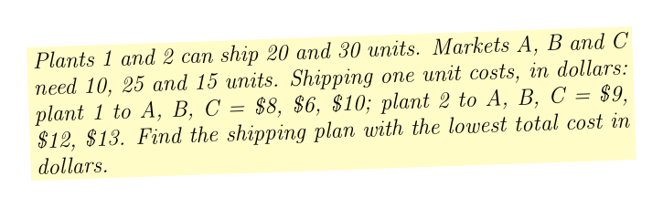
The problem
Plants 1 and 2 can ship 20 and 30 units. Markets A, B and C need 10, 25 and 15 units. Shipping one unit costs, in dollars: plant 1 to A, B, C = $8, $6, $10; plant 2 to A, B, C = $9, $12, $13. Find the shipping plan with the lowest total cost in dollars.
How the model was built
The objective as written from the problem, before the numbers are multiplied out:
The model
Each line has a plain-language note on the right.
| make as small as possible: total shipping cost (dollars) | |
| limit 1: left side cannot exceed 20 | |
| limit 2: left side cannot exceed 30 | |
| limit 3: left side must reach at least 10 | |
| limit 4: left side must reach at least 25 | |
| limit 5: left side must reach at least 15 | |
| units shipped from plant 1 to market A (units) cannot be negative | |
| units shipped from plant 1 to market B (units) cannot be negative | |
| units shipped from plant 1 to market C (units) cannot be negative | |
| units shipped from plant 2 to market A (units) cannot be negative | |
| units shipped from plant 2 to market B (units) cannot be negative | |
| units shipped from plant 2 to market C (units) cannot be negative |
In matrix form
With its numbers:
What is being decided
There are 6 decision variables.
| Variable | Type | Meaning |
|---|---|---|
| x1A | real number | units shipped from plant 1 to market A (units) |
| x1B | real number | units shipped from plant 1 to market B (units) |
| x1C | real number | units shipped from plant 1 to market C (units) |
| x2A | real number | units shipped from plant 2 to market A (units) |
| x2B | real number | units shipped from plant 2 to market B (units) |
| x2C | real number | units shipped from plant 2 to market C (units) |
Goal and limits
Minimize total shipping cost (dollars) subject to 11 constraints, of which 6 are simple bounds on a single variable.
Problem type
LP, complexity level 2: a linear program. Solved with HIGHS at the Medium solver tier.
The answer at a glance
The optimal value of each decision, as the solver returned it.
Which constraints hold the answer in place
Binding (no slack left): constraints 1, 2, 3, 4, 5, 6, 8 (see the table). Changing a binding constraint changes the answer; a slack one can move a little without effect.
| # | Constraint | Value | Limit | Slack | Binding |
|---|---|---|---|---|---|
| 1 | x1A + x1B + x1C <= 20 | 20 | 20 | 0 | yes |
| 2 | x2A + x2B + x2C <= 30 | 30 | 30 | 0 | yes |
| 3 | x1A + x2A >= 10 | 10 | 10 | 0 | yes |
| 4 | x1B + x2B >= 25 | 25 | 25 | 0 | yes |
| 5 | x1C + x2C >= 15 | 15 | 15 | 0 | yes |
| 6 | x1A >= 0 | 0 | 0 | 0 | yes |
| 7 | x1B >= 0 | 20 | 0 | 20 | |
| 8 | x1C >= 0 | 0 | 0 | 0 | yes |
| 9 | x2A >= 0 | 10 | 0 | 10 | |
| 10 | x2B >= 0 | 5 | 0 | 5 | |
| 11 | x2C >= 0 | 15 | 0 | 15 |
Why this is optimal
A proof you can check by hand. Multiply each constraint in the table by its weight and add them up: the result is a lower limit on the objective that holds for every plan meeting the constraints. Our answer reaches that limit exactly, so no plan does better. A negative weight turns a limit around (for example ≥ into ≤) before adding. Every step was checked in exact fractions, not rounded decimals.
| # | Constraint | Weight |
|---|---|---|
| 1 | x1A + x1B + x1C ≤ 20 | -6 |
| 3 | x1A + x2A ≥ 10 | 9 |
| 4 | x1B + x2B ≥ 25 | 12 |
| 5 | x1C + x2C ≥ 15 | 13 |
Algebraic model (low level)
Decision variables, objective and every constraint written out; this is exactly what the solver receives.
Standard form
As a linear program: minimize cᵀx subject to A x ≤ b (the inequality rows) and A_eq x = b_eq (the equations); a maximization is written as minimizing the negative.
Model code (cvxpy)
The same model in cvxpy, ready to run.
import cvxpy as cp

x1A = cp.Variable(name='x1A')  # units shipped from plant 1 to market A (units)
x1B = cp.Variable(name='x1B')  # units shipped from plant 1 to market B (units)
x1C = cp.Variable(name='x1C')  # units shipped from plant 1 to market C (units)
x2A = cp.Variable(name='x2A')  # units shipped from plant 2 to market A (units)
x2B = cp.Variable(name='x2B')  # units shipped from plant 2 to market B (units)
x2C = cp.Variable(name='x2C')  # units shipped from plant 2 to market C (units)

objective = cp.Minimize(8*x1A + 6*x1B + 10*x1C + 9*x2A + 12*x2B + 13*x2C)
constraints = [
    x1A + x1B + x1C <= 20,
    x2A + x2B + x2C <= 30,
    x1A + x2A >= 10,
    x1B + x2B >= 25,
    x1C + x2C >= 15,
    x1A >= 0,
    x1B >= 0,
    x1C >= 0,
    x2A >= 0,
    x2B >= 0,
    x2C >= 0,
]
problem = cp.Problem(objective, constraints)
problem.solve(solver='HIGHS')
print(problem.status, problem.value)
print('x1A =', x1A.value)
print('x1B =', x1B.value)
print('x1C =', x1C.value)
print('x2A =', x2A.value)
print('x2B =', x2B.value)
print('x2C =', x2C.value)
The dual problem
Every constraint of the original (primal) problem gets a price, and every primal variable becomes a constraint on those prices. Strong duality: primal and dual optima are equal (465).
| Dual variable | Prices | Value |
|---|---|---|
| y1 | price of constraint 'x1A + x1B + x1C <= 20' (objective change per extra unit of its right-hand side) | -6 |
| y2 | price of constraint 'x2A + x2B + x2C <= 30' (objective change per extra unit of its right-hand side) | 0 |
| y3 | price of constraint 'x1A + x2A >= 10' (objective change per extra unit of its right-hand side) | 9 |
| y4 | price of constraint 'x1B + x2B >= 25' (objective change per extra unit of its right-hand side) | 12 |
| y5 | price of constraint 'x1C + x2C >= 15' (objective change per extra unit of its right-hand side) | 13 |
Solve your own
This is the model as the app reads it. Change any number and solve it in the free box on the front page (no account needed).
minimize 8*x1A + 6*x1B + 10*x1C + 9*x2A + 12*x2B + 13*x2C
subject to
x1A + x1B + x1C <= 20   # plant 1 capacity (units)
x2A + x2B + x2C <= 30   # plant 2 capacity (units)
x1A + x2A >= 10   # market A demand (units)
x1B + x2B >= 25   # market B demand (units)
x1C + x2C >= 15   # market C demand (units)
x1A, x1B, x1C, x2A, x2B, x2C >= 0
# x1A = units shipped from plant 1 to market A (units)
# x1B = units shipped from plant 1 to market B (units)
# x1C = units shipped from plant 1 to market C (units)
# x2A = units shipped from plant 2 to market A (units)
# x2B = units shipped from plant 2 to market B (units)
# x2C = units shipped from plant 2 to market C (units)
# objective = total shipping cost (dollars)Checked: the app's answer matches the reference answer in our test set, which two solvers (HIGHS, CLARABEL) agree on. Built 2026-11-17.
Related examples
Try ProvenDecisions free: type, photograph or say an optimization problem; every answer is checked by a solver.